
Nine attention variants, one Pareto plot
What an H100, 30 million parameters, and a few hours of training had to say about MHA, MQA, GQA, and MLA.

I had nine 30-million-parameter transformers, an H100, and a question I want to answer: how much KV cache do I actually need to spend per percent of validation loss?
So I trained them all. Same data, same number of steps, same dropout, same optimizer, same RoPE configuration. Different attention. Then I put them on a single chart and let the numbers decide.
This is what came out.
(This is part one of a series on KV-cache economics the same thread as my earlier deep-dive on vLLM serving knobs on H100s. There, I treated the KV cache as a serving-time constraint. Here, I go one level down: the architecture decision that sets the size of that cache in the first place.)

The setup
Nine decoder-only transformers, all 30M parameters give or take a million, all trained on the same TinyStories slice for 3,000 steps. The only thing that changed across runs was the attention layer.
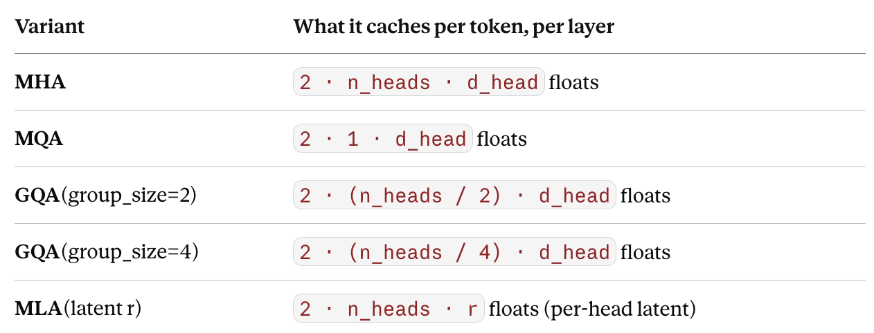
For MLA I tested five compression ratios: r ∈ {d_head, d_head/2, d_head/4, d_head/8, d_head/16}. With my model d_head = 48 that’s r ∈ {48, 24, 12, 6, 3}. The smallest is enough to be properly aggressive; not enough to break the model entirely.
Architecture details that matter:
d_model = 384, n_heads = 8, n_layers = 6, so d_head = 48
max_seq_len = 256, batch size 64
AdamW, lr 3e-4, cosine schedule with 200 warmup steps
RoPE on every variant (applied to Q and K; for MLA, on the up-projected K)
bf16 inference, fp32 training
All nine trained checkpoints are public on Hugging Face, alongside the raw benchmark CSVs. Poke at them.
I’m not pretending this scale gives the final word on attention. It gives a controlled answer at this scale and a methodology you can paste over your own setup.
The headline plot
Validation perplexity against KV cache footprint at the largest batch and longest context I tested (batch=16, ctx=32k). Lower-left wins.
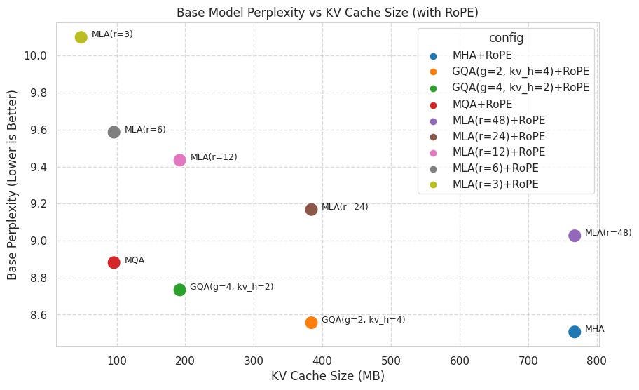
The frontier is short: MQA → GQA(g=4) → GQA(g=2) → MHA, walking from smallest cache to lowest loss. Every MLA configuration sits above this line.
Here’s the same data as a table, sorted by val loss:
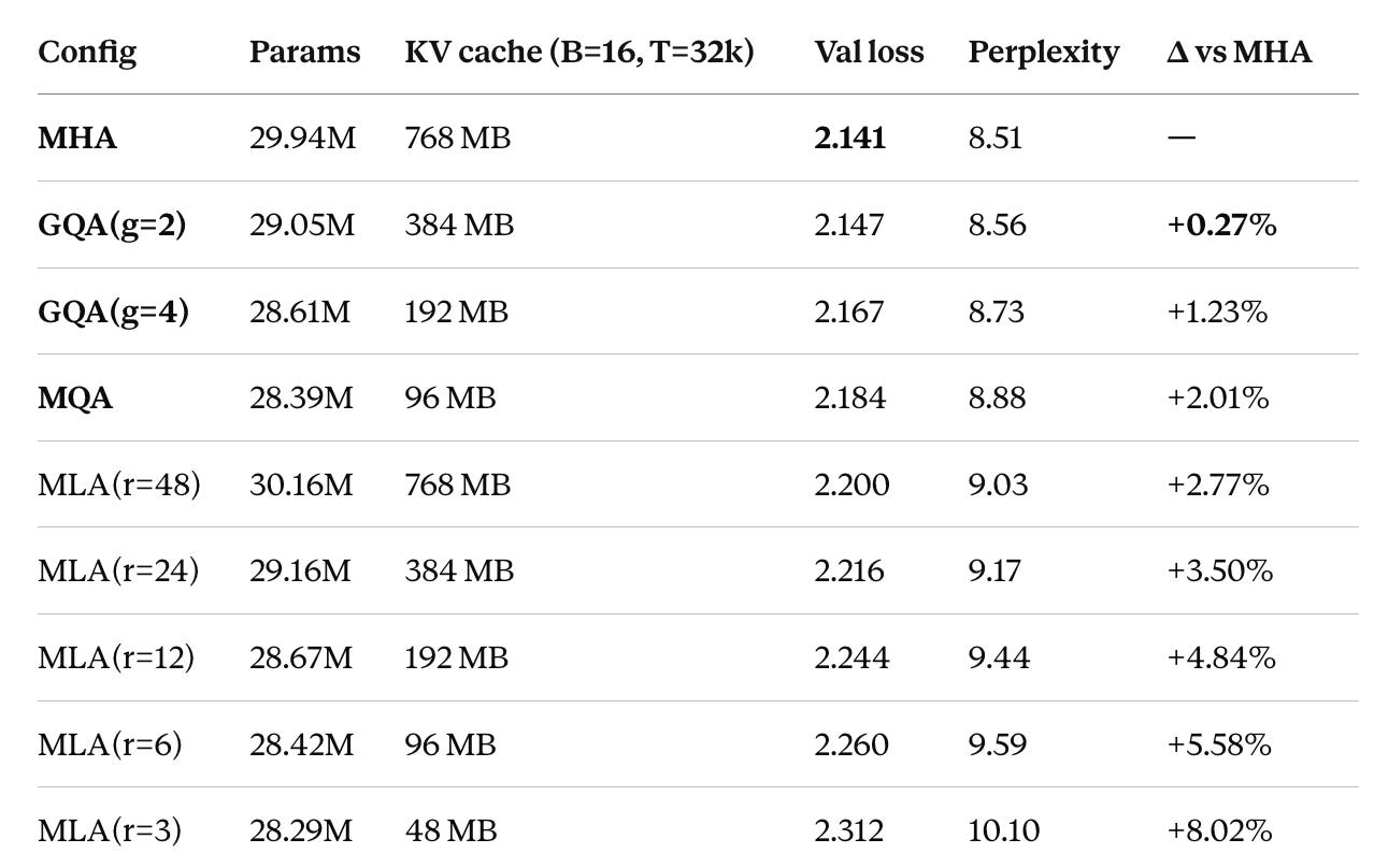
(Δ is % of validation loss, not perplexity in perplexity terms GQA(g=2)’s gap is 0.59%. I’ll use val loss throughout since it’s the metric the optimizer sees.)
A few things jump out.
One: GQA(g=2) gives up 0.006 nats of val loss for half the cache. That is not a typo. Cutting the cache in half costs you a quarter of one percent of validation loss.
Two: at every cache budget I tested, the simpler architecture wins on quality. MHA beats MLA(r=48) at 768 MB. GQA(g=2) beats MLA(r=24) at 384 MB. GQA(g=4) beats MLA(r=12) at 192 MB. MQA beats MLA(r=6) at 96 MB. The gap is consistently ~3% of val loss.
Three: the MLA latent isn’t free. At full rank (r = d_head), MLA caches the same number of bytes as MHA but trains to a higher loss. The extra projections aren’t paying for themselves at this scale.
I also scored generation-quality proxies on samples from every checkpoint distinct-1/distinct-2 diversity and perplexity under a reference model. Neither showed systematic degradation across configs; they bounce around within noise while val loss separates cleanly. At this scale, val loss is the discriminating metric, which is why it anchors the chart.
Why the simpler architectures win at small scale
I want to resist over-explaining a result, but here’s the mechanistic story I find consistent with what I see.
KV-cache compression has two flavors. Head-sharing (MQA / GQA) reduces the number of distinct keys and values by tying heads together. Rank compression (MLA) keeps per-head representations but factors them through a low-dimensional latent.
Head-sharing is a hard constraint on representation diversity and you literally have fewer keys. Rank compression is a softer constraint, but it adds parameters (the up-projection) and its expressive ceiling depends on whether the data actually benefits from per-head specialization within the latent subspace.
At 30M parameters on TinyStories, the model has more representational room than it knows what to do with. Heads are correlated. Tying them together (MQA / GQA) costs almost nothing because they were doing similar work anyway. Compressing them through a latent (MLA) loses information because the up-projection is a learned filter that takes capacity to fit, and capacity isn’t the bottleneck, the data is.
This is an argument for why the MLA penalty might shrink as model and dataset scale up: when heads are differentiated and capacity becomes the bottleneck, the latent’s filtering effect can become a feature instead of a tax. I haven’t tested that here. I’m noting the conjecture.
What this looks like in production-scale dimensions
The 30M-parameter ablation is the trained part. To see what these architectures look like at LLM-deployment scale, I ran a separate compute-only benchmark with synthetic tensors at n_heads=32, d_head=128, the dimensions of a Llama-7B-class model, across batch sizes up to 16 and contexts up to 131,072.
That benchmark isn’t trained, so it has nothing to say about quality. But it tells you what the cache itself does:
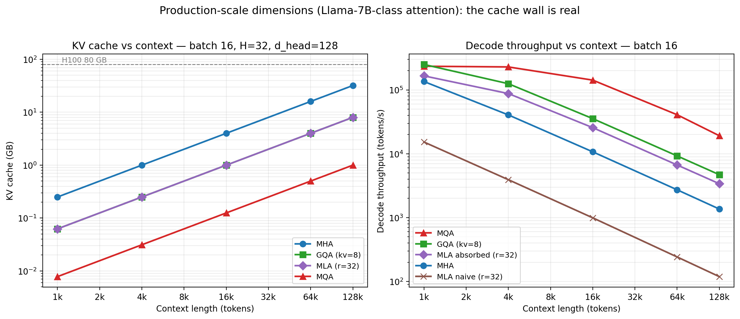
Left: KV cache vs context at batch 16. MHA crosses 32 GB at 128k against an 80 GB card; GQA(kv=8) and MLA(r=32) overlap at 8 GB (the purple diamond sits on the green square); MQA stays at 1 GB.
Right: decode throughput. Note the brown line at the bottom. That’s naive MLA, and it’s the subject of the next post.
At batch=16, ctx=131k:
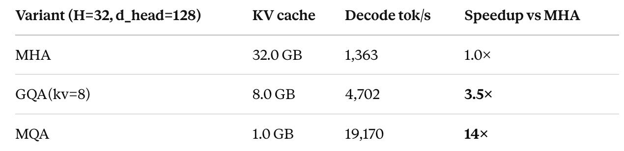
The cache wall isn’t theoretical. On an 80 GB H100, MHA’s 32 GB KV cache leaves you 48 GB for everything else: model weights, activations, batch parallelism. You can squeeze it in. You can’t serve with it.
GQA’s 4× cache reduction is the practical engineering decision. MQA’s 14× speedup at long context is the throughput-king answer for read-heavy workloads.
The MLA story isn’t quite over
There’s a subtlety I owe you, because it would otherwise look like I’m dismissing MLA outright.
MLA’s decode step has two flavors. The naive form caches the per-head latent K_lat, then at every decode step reconstructs the full K = K_lat · W_k_up before doing attention. This is what most first implementations write, and it’s an order of magnitude slower than MHA at long context. The kernel is doing all the work of MHA plus the latent up-projection over the entire cache. That’s the brown line dying at the bottom of Figure 2.
The absorbed form is mathematically identical but computationally different. Notice that:
score[t] = q · k[t]ᵀ = q · (k_lat[t] · W_k_up)ᵀ = (q · W_k_upᵀ) · k_lat[t]ᵀ
You can fold W_k_up into Q at model-load time. Now decode never reconstructs K attention runs against the cached latent directly. Same cache shape, same numerics, dramatically smaller per-step work.
In my benchmarks, absorbed MLA at the same compression ratio is 30× faster than naive MLA at 128k context. It pulls MLA’s decode latency from “unusable” to “competitive with MHA.”
That makes two things true at once:
On the quality-per-byte axis (this article), MLA is dominated by GQA at every cache budget I tested.
On the latency axis, absorbed MLA can close the throughput gap to MHA and beat it at long context, where MHA goes bandwidth-bound.
The implementation choice matters as much as the architecture choice. I’ll dig into absorbed MLA in the next post.
What the data does not say
Six caveats so this isn’t read for more than it claims:
Scale. 30M parameters is small. The story can change at 1B, 7B, 70B. There’s a real possibility that MLA’s expressive ceiling lifts above GQA’s once heads start carrying differentiated information. Worth re-running.
Domain. TinyStories has constrained vocabulary and narrative structure. Code, technical text, multilingual data, math, none of it tested.
Training duration. 3,000 steps. Loss curves are still trending downward at the final step. A longer run might widen or narrow the gaps.
MLA flavor. I implemented per-head latent with naive RoPE on the up-projected K. DeepSeek-V2 uses a shared latent across heads with a decoupled RoPE path, which is more parameter-efficient and preserves absorbed-decode through RoPE. I’d expect that flavor to land closer to GQA on the quality axis. In fact, my result is consistent with why DeepSeek needed decoupled RoPE in the first place.
Cache reading reality. My production-scale numbers are decode-step-only, not full forward passes. Multiply latency by
n_layersfor a real serving estimate.One seed. I ran one training seed per config. The variance is small relative to the gaps, but I should rerun with three seeds before publishing anything stronger than “in this setup.”
What I’m taking away
A working default:
For a small-to-mid LM where you can afford half of MHA’s KV cache, use GQA with group size 2. Quality drops by 0.3% and you get the cache savings for free.
If your serving environment is bandwidth-bound (long context, large batch), use MQA. The 8× cache reduction is worth the ~2% quality cost, and it dominates throughput at long context.
Reach for MLA when you’ve measured your specific workload and have a reason to believe the per-head latent recovers something head-sharing can’t. At small scale, in my testing, that wasn’t the case.
The methodology takeaway is more important than the architecture choice: architecture decisions are workload decisions in disguise. Don’t pick attention from a benchmark someone else ran on a model that isn’t yours, on data you don’t share, at a context length you don’t serve. Train three configs on your data for an afternoon. Plot val loss against KV cache. Pick from your own Pareto frontier.
Reproduce it
Everything in this post is free and public:
Trained checkpoints (all 9):
genaiquest/tinystories-attn-ablations-v2Raw data: the 9-row quality table and 210 compute-benchmark cells
Harness: the training and benchmark code
If you rerun any of this on your own data or at larger scale, I genuinely want to see the numbers, especially if they disagree with mine.
What’s next in this series
Absorbed MLA, properly benchmarked. The decode-time speedup is dramatic enough to deserve its own post, one matrix identity, 30× at 128k context. That’s article two, next week.
A decision tree for picking attention. Given context length, batch size, and quality budget, what’s the right choice? 210 benchmark cells → a flowchart you can save. Article three.
What does RoPE actually cost? I ran the entire benchmark suite a second time without RoPE. The answer interacts with everything above. Later in the series.
Subscribe to get each article when it drops.
I lead agentic AI engineering (consumer-scale conversational agents, LLMOps, evaluation infrastructure) and spent the last two decades shipping ML systems at Apple, Twitter, Shopify, and three startups. This post is part of an ongoing series on efficient agentic AI. Find me on LinkedIn. Part one of the series: