
The MLA decode speedup hiding in your model card
Naive MLA is an order of magnitude slower than MHA at long context. The fix is one matrix identity and almost nobody writes it the first time.

I had a benchmarking puzzle.
I’d implemented Multi-Head Latent Attention from the obvious read of the description: cache a low-rank latent, reconstruct full keys and values at decode time, run attention. Same architecture, smaller cache. Cache savings should buy faster decode. Right?
Wrong. At 32K context with batch=16, my MLA was decoding at 5,000 tokens per second. My MHA at the same setup was doing 42,000.
MLA had a smaller cache and was 8× slower.
That ratio bothered me for two days. The architecture is supposed to be a Pareto improvement that’s the whole pitch. The numbers said the opposite. Either the paper was wrong about something fundamental, or I’d written the wrong implementation. The latter is overwhelmingly more likely when you’re debugging your own code, so I went looking.
I found a math identity that, applied at model-load time, makes MLA decode at 71,000 tokens per second with the same cache. Thirteen times faster. Same numerics, same outputs. One change.
This is that identity. And the reason most first MLA implementations leave a ~30× speedup on the table.
(Part two of the KV-cache economics series. Part one, nine attention variants on one Pareto plot, found MLA quality-dominated by GQA at 30M scale. This post is about the other axis: why MLA’s latency reputation is an implementation artifact.)

The naive form, written out
Here’s MLA’s decode step the way you write it the first time:
def naive_mla_decode_step(q, k_lat, v_lat, W_k_up, W_v_up):
    """One decode step. q: (B,H,1,d). k_lat,v_lat: (B,H,T,r). W_*_up: (H,r,d)."""
    # 1. Up-project the cached latents to full key and value.
    K = torch.einsum("bhtr,hrd->bhtd", k_lat, W_k_up)   # (B, H, T, d)
    V = torch.einsum("bhtr,hrd->bhtd", v_lat, W_v_up)   # (B, H, T, d)
    # 2. Standard attention.
    scores = q @ K.transpose(-2, -1) / sqrt(d)          # (B, H, 1, T)
    probs  = scores.softmax(-1)
    return probs @ V                                    # (B, H, 1, d)
Two big matmuls before attention even starts. Each one runs over the entire cache, every cached token, every head. The dominant FLOP cost is O(B · H · T · r · d_head), proportional to T · r · d_head.
That T is the killer. For every new decode step, you’re redoing work over the full cached past. Doubling the context doubles the per-step cost. This is why naive MLA’s latency curve goes from 0.15 ms at 1K context to 3 ms at 32K, a 20× increase for a 32× context increase. The cost is in the up-projection, not the attention.
The identity
Standard scaled-dot-product attention computes, for each cached position t:
score[t] = q · K[t]ᵀIn MLA, K[t] = K_lat[t] · W_k_up. Substituting:
score[t] = q · (K_lat[t] · W_k_up)ᵀ
         = q · W_k_upᵀ · K_lat[t]ᵀ
         = (q · W_k_upᵀ) · K_lat[t]ᵀ
That last regrouping is the whole insight. The product q · W_k_upᵀ doesn’t depend on t. Compute it once per decode step, outside the loop over cached tokens and then run attention against the cached latent directly.
Define:
q' = q · W_k_upᵀ # shape: (B, H, 1, r)And attention becomes:
score[t] = q' · K_lat[t]ᵀq' is small. K_lat is what we already had cached. The full key reconstruction never happens.
For V it’s almost the same trick, applied after attention:
out_lat = probs · V_lat       # in latent space, shape: (B, H, 1, r)
out     = out_lat · W_v_up    # project back to head dim, shape: (B, H, 1, d_head)
You compute attention’s weighted sum in latent space, then project once at the end. V is also never reconstructed.
The absorbed form
Here’s the decode step rewritten:
def absorbed_mla_decode_step(q, k_lat, v_lat, W_k_up, W_v_up):
    """One decode step. Same I/O as naive — different math, dramatically faster."""
    # 1. Absorb W_k_up into Q. O(H * r * d_head). NOT a function of T.
    q_abs = torch.einsum("bhtd,hrd->bhtr", q, W_k_up)   # (B, H, 1, r)
    # 2. Attention runs against the latent K directly.
    scores = q_abs @ k_lat.transpose(-2, -1) / sqrt(d)  # (B, H, 1, T)
    probs  = scores.softmax(-1)
    # 3. Aggregate in latent space, then project out.
    out_lat = probs @ v_lat                             # (B, H, 1, r)
    return torch.einsum("bhtr,hrd->bhtd", out_lat, W_v_up)
What changed:
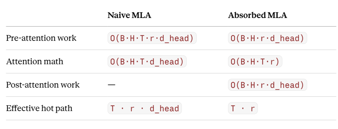
The hot path lost a factor of d_head. With d_head = 128 (production scale), that’s the difference between “barely usable” and “competitive.”
What the numbers actually look like
I ran both forms on an H100 across a context-length sweep, batch=16, in bf16.
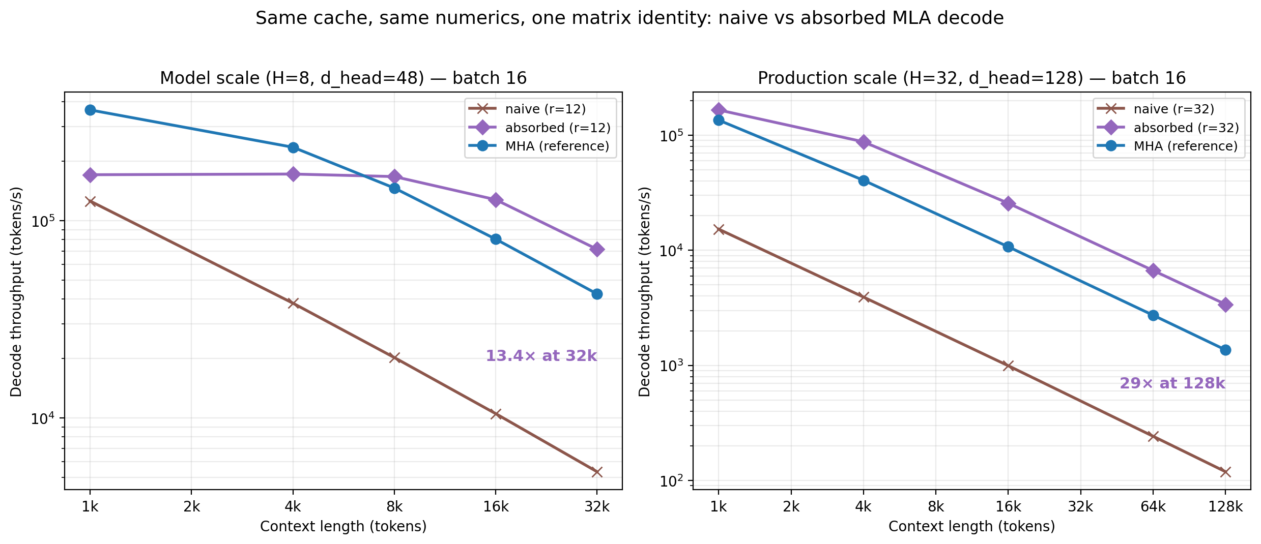
Naive vs absorbed MLA decode throughput, with MHA as reference. Left: my model's dimensions. Right: Llama-7B-class dimensions. Two things to notice: the absorbed line sits 13–29× above the naive line at long context, and at model scale it crosses above MHA past ~8k. Once you're bandwidth-bound, the smaller latent cache reads fewer bytes per step than MHA's full KV. (Absorbed runs are benchmarked without RoPE on K, see "the catch" below for why that matters.)
At my model’s dimensions (H=8, d_head=48):
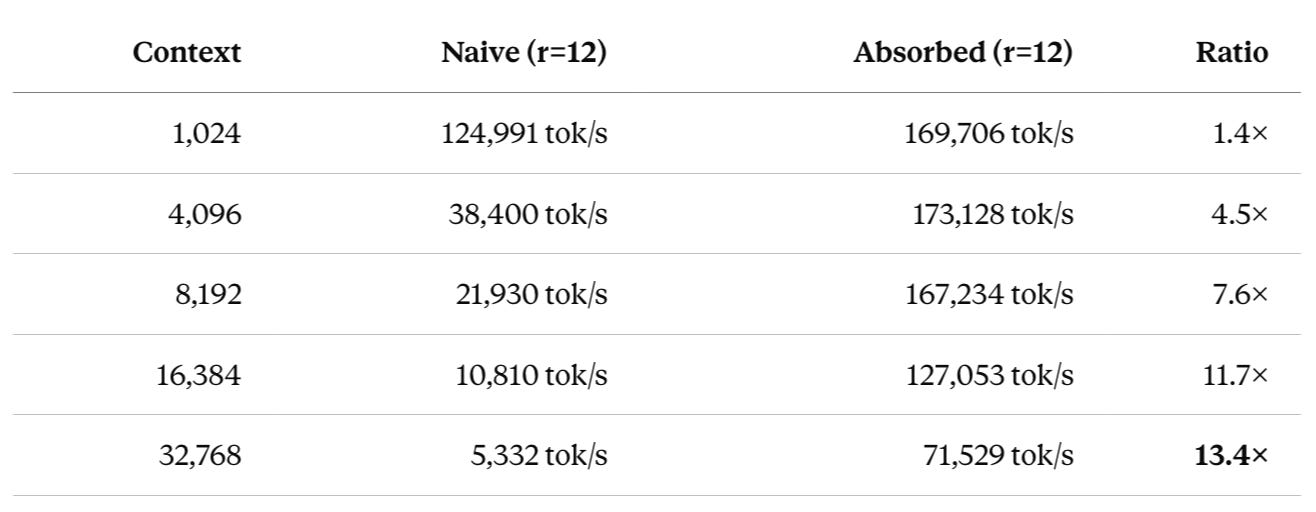
The ratio grows with context because the naive form’s T · r · d_head cost grows linearly with T while the absorbed form’s T · r cost grows... still linearly with T, but with a small constant.
At production-scale dimensions (H=32, d_head=128, latent r=32, batch=16):
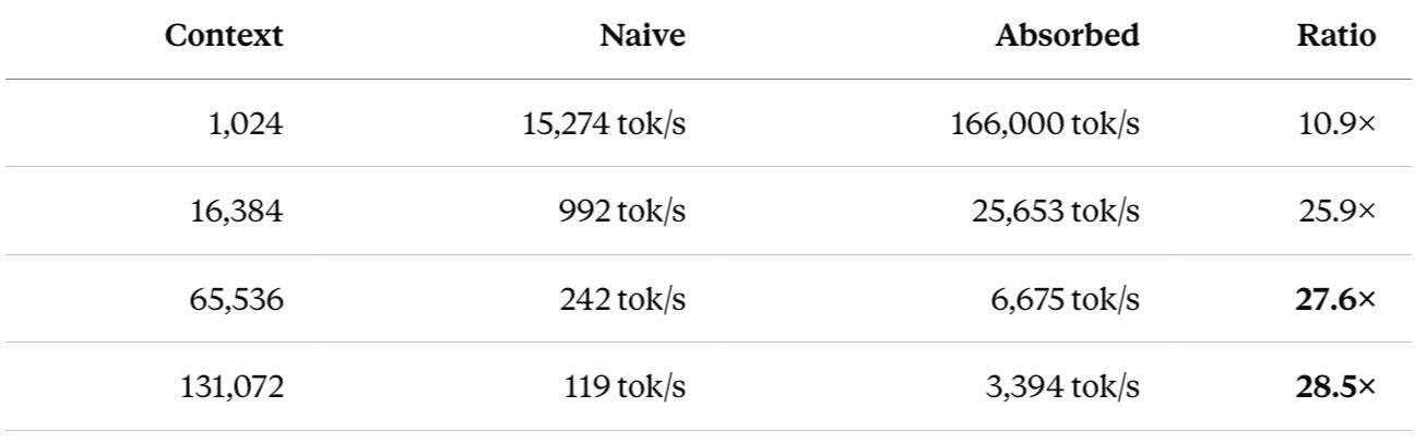
Almost 30× at 128K context. That’s the difference between “you wouldn’t ship this” and “this is genuinely competitive with GQA.”
Where absorbed MLA actually lands
Absorbed MLA fixes MLA’s decode cost. It doesn’t make MLA the answer. Here’s the full picture at production scale, batch=16, ctx=131K:
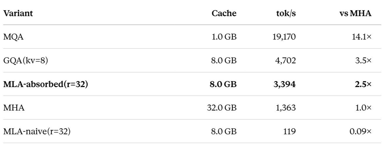
Absorbed MLA at the same cache footprint as GQA(kv=8) is about 27% slower than GQA. That’s the realistic competitive position. MQA still dominates because its cache is 8× smaller, and at long context the dominant cost is reading bytes, not doing math.
What absorbed MLA does offer that GQA doesn’t:
The latent representation is per-head, so you preserve some head-specific structure that GQA’s hard tying loses.
It’s a continuous knob (
r), not a discrete one (group_sizedividesn_heads), so you have more granularity in the cache-vs-quality trade.
Whether either of those matters in your workload is an empirical question, not a theoretical one. Run it.
The catch nobody tells you about
Absorbed MLA only works cleanly if W_k_up is the only thing you fold into Q. Add RoPE on K and the absorption breaks.
Why? RoPE is position-dependent. If your real key is K[t] = RoPE_t(K_lat[t] · W_k_up), you can’t push W_k_upᵀ through RoPE_t because RoPE applies a different rotation per position. The factorization doesn’t hold.
There are two ways out.
One: apply RoPE to the up-projected K at every decode step (what I do in the trained-quality side of my work). This loses the absorbed-decode trick. Latency goes back up.
Two: decoupled RoPE, what DeepSeek-V2 does. Add a separate small per-head key with RoPE applied, cached alongside the latent. Concatenate scores from the latent path (no RoPE, absorbable) and the small RoPE path (positional, not absorbable). The absorbable part stays absorbable; the small RoPE path adds a fixed-cost per-step matmul that doesn’t grow with r.
Decoupled RoPE is the right answer for production-grade MLA. It’s a bit more engineering and a bit more cache, but it preserves both the position information and the absorbed-decode speed. I haven’t trained that flavor yet, it’s on my list, but the math is straightforward.
(And if you’re wondering “how much quality is RoPE even worth?” I re-ran the entire ablation suite without positional encoding to answer exactly that. The answer is a bigger number than the whole MHA-vs-GQA debate. Later in this series.)
What this means for the field’s MLA discourse
A take I see frequently in serving discussions: “MLA is theoretically interesting but slow in practice.”
Half right. The theoretical interest is real. The practical slowness is an implementation choice. In benchmarks where MLA looks 10× slower than MHA, the comparison is almost always against the naive decode form. Absorbed MLA closes most of that gap.
If you’re evaluating MLA for production:
Implement absorbed decode from day one. It’s the same code path with two different einsums. The naive form is for understanding the math, not for shipping.
Use decoupled RoPE if you need positional encoding. The absorbed form composes with content-only K and positional structure goes through a separate small head.
Measure on your workload. Cache savings only convert into latency savings when memory bandwidth is the dominant cost, long context, large batch. Below that regime, you may be FLOP-bound and the simpler architectures win on Math-FLOPs-per-byte intensity.
Caveats
These are decode-only benchmarks. Prefill cost is different and the absorbed form helps less there (the up-projection cost amortizes over prefill in a way it doesn’t over per-step decode).
Numbers are bf16, single H100, single layer. Multiply latencies by
n_layersfor full-model decode time.I’m running PyTorch’s default SDPA backends. A custom CUDA kernel for absorbed MLA could squeeze further gains; a quick search of the public ecosystem suggests this is mostly an inference-framework problem, not a research one.
Cache reconstruction in naive MLA was implemented with
torch.einsum. A more aggressive implementation might fuse it with attention; I expect the gap to shrink, not vanish.
Reproduce it
Both decode kernels (naive and absorbed), the full benchmark harness, and every CSV behind the tables above are free and public:
Code + data: [Request for access]
Trained checkpoints from part one:
genaiquest/tinystories-attn-ablations-v2
What I’d test next
Absorbed MLA + decoupled RoPE. Train it. See if it lands on the Pareto frontier with GQA, or above.
Quantized absorbed MLA. int8 latent + bf16 weights. The latent is the cache; quantizing it stacks with the architectural compression.
Larger scale. At 7B or 70B, the latent’s expressive role might change. MLA may finally pay for its extra projections.
I lead agentic AI engineering (consumer-scale conversational agents, LLMOps, evaluation infrastructure) and spent the last two decades shipping ML systems at Apple, Twitter, Shopify, and three startups. This is Article two of the KV-cache economics series. Article three next week: A decision tree for picking attention from your context length, batch size, and quality budget. Backed by 210 benchmark cells. Find me on LinkedIn.
Earlier:
